[1]:
import matplotlib.pyplot as plt
import numpy as np
from mabwiser.mab import LearningPolicy

from alns import ALNS
from alns.accept import *
from alns.select import *
from alns.stop import *
[2]:
%matplotlib inline
[3]:
SEED = 42
[4]:
np.random.seed(SEED)
ALNS features
The alns package offers a number of different operator selection schemes, and acceptance and stopping criteria. In this notebook, we show some these in action solving a toy knapsack problem. Along the way we explain how they work, and show how you can use them in your ALNS heuristic.
In our toy 0/1-knapsack problem, there are \(n = 100\) items \(i\) with profit \(p_i > 0\) and weight \(w_i > 0\). The goal is to find a subset of the items that maximizes the profit, while keeping the total weight below a given limit \(W\). The problem then reads follows:
subject to
First we quickly set up everything required for solving the problem with ALNS. In particular, we define a solution state, and a few destroy and repair operators. Our goal is not to solve this problem very well, so we set up only the bare minimum needed to get the ALNS algorithm going.
[5]:
n = 100
p = np.random.randint(1, 100, size=n)
w = np.random.randint(10, 50, size=n)
W = 1_000

# Percentage of items to remove in each iteration
destroy_rate = 0.25
[6]:
class KnapsackState:
    """
    Solution class for the 0/1 knapsack problem. It stores the current
    solution as a vector of binary variables, one for each item.
    """

    def __init__(self, x: np.ndarray):
        self.x = x

    def objective(self) -> int:
        # Negative p since ALNS expects a minimisation problem.
        return -p @ self.x

    def weight(self) -> int:
        return w @ self.x
Destroy operators
We implement two operators:
A simple random destroy operator, which removes items from the knapsack at random.
A destroy operator that removes items based on their relative merits, that is, for an item \(i\) currently in the knapsack, it removes those whose \(p_i / w_i\) values are smallest.
[7]:
def to_destroy(state: KnapsackState) -> int:
    return int(destroy_rate * state.x.sum())
[8]:
def random_remove(state: KnapsackState, rng):
    probs = state.x / state.x.sum()
    to_remove = rng.choice(np.arange(n), size=to_destroy(state), p=probs)

    assignments = state.x.copy()
    assignments[to_remove] = 0

    return KnapsackState(x=assignments)
[9]:
def worst_remove(state: KnapsackState, rng):
    merit = state.x * p / w
    by_merit = np.argsort(-merit)
    by_merit = by_merit[by_merit > 0]
    to_remove = by_merit[: to_destroy(state)]

    assignments = state.x.copy()
    assignments[to_remove] = 0

    return KnapsackState(x=assignments)
Repair operators
We implement only the random repair operator. The focus of this notebook is not on solving the knapsack problem very well, but rather to showcase the different operator schemes and acceptance criteria.
[10]:
def random_repair(state: KnapsackState, rng):
    unselected = np.argwhere(state.x == 0)
    rng.shuffle(unselected)

    while True:
        can_insert = w[unselected] <= W - state.weight()
        unselected = unselected[can_insert]

        if len(unselected) != 0:
            insert, unselected = unselected[0], unselected[1:]
            state.x[insert] = 1
        else:
            return state
ALNS
[11]:
def make_alns() -> ALNS:
    rng = np.random.default_rng(SEED)
    alns = ALNS(rng)

    alns.add_destroy_operator(random_remove)
    alns.add_destroy_operator(worst_remove)

    alns.add_repair_operator(random_repair)

    return alns
[12]:
# Terrible - but simple - first solution, where only the first item is
# selected.
init_sol = KnapsackState(np.zeros(n))
init_sol.x[0] = 1
Operator selection schemes
We now have everything set-up for solving the problem. We will now look at several of the operator selection schemes the alns package offers. The list is not exhaustive: for a complete overview, head over to alns.select in the documentation.
Here, we use the HillClimbing acceptance criterion, which only accepts better solutions.
[13]:
accept = HillClimbing()
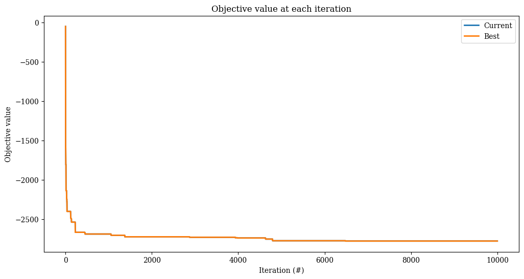
Roulette wheel
The RouletteWheel scheme updates operator weights as a convex combination of the current weight, and the new score.
When the algorithm starts, all operators \(i\) are assigned weight \(\omega_i = 1\). In each iteration, a destroy and repair operator \(d\) and \(r\) are selected by the ALNS algorithm, based on the current weights \(\omega_i\). These operators are applied to the current solution, resulting in a new candidate solution. This candidate is evaluated by the ALNS algorithm, which leads to one of four outcomes:
The candidate solution is a new global best.
The candidate solution is better than the current solution, but not a global best.
The candidate solution is accepted.
The candidate solution is rejected.
Each of these four outcomes is assigned a score \(s_j~\) (with \(j = 1,...,4\)). After observing outcome \(j\), the weights of the destroy and repair operator \(d\) and \(r\) that were applied are updated as follows:
where \(0 \le \theta \le 1\) (known as the operator decay rate) is a parameter.
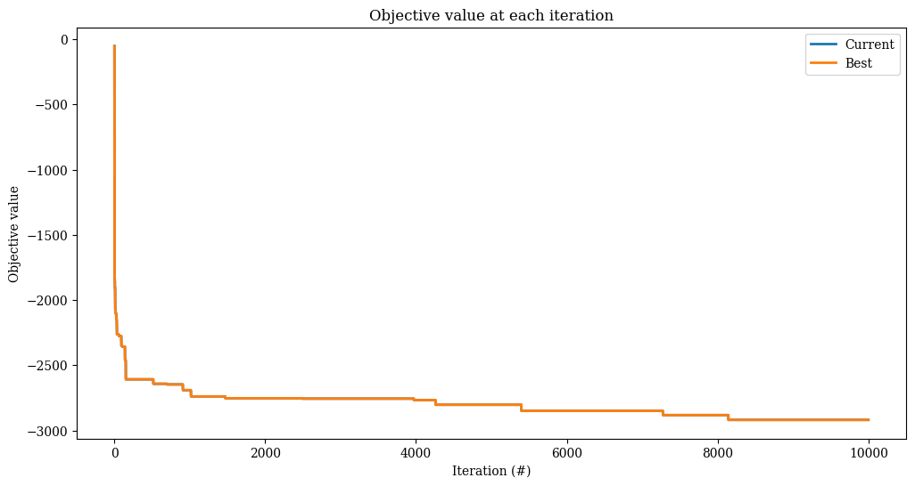
[14]:
select = RouletteWheel(
    scores=[5, 2, 1, 0.5], decay=0.8, num_destroy=2, num_repair=1
)

alns = make_alns()
res = alns.iterate(init_sol, select, accept, MaxIterations(10_000))

print(f"Found solution with objective {-res.best_state.objective()}.")
Found solution with objective 2863.0.
[15]:
_, ax = plt.subplots(figsize=(12, 6))
res.plot_objectives(ax=ax, lw=2)
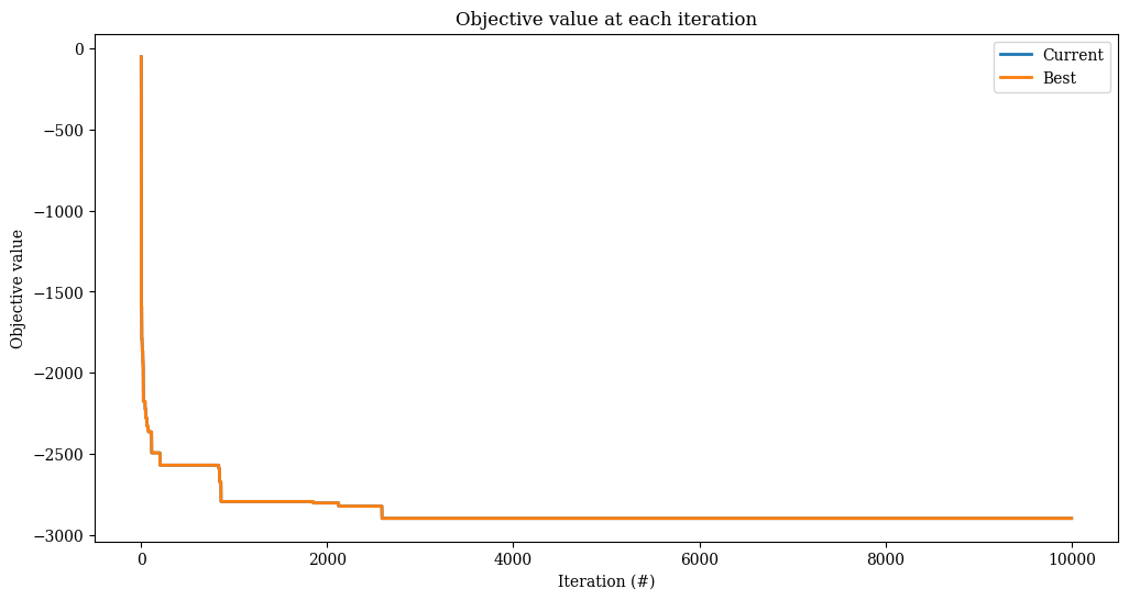
Segmented roulette wheel
The RouletteWheel scheme continuously updates the weights of the destroy and repair operators. As a consequence, it might overlook that different operators are more effective in the neighbourhood of different solutions.
The SegmentedRouletteWheel scheme attempts to fix this, by fixing the operator weights \(\omega_i\) for a number of iterations (the segment length). Initially, all weights are set to one, as in RouletteWheel. A separate score is tracked for each operator \(d\) and \(r\), to which the observed scores \(s_j\) are added in each iteration where \(d\) and \(r\) are applied. After the segment concludes, these summed scores are added to the weights \(\omega_i\) as
a convex combination using a parameter \(\theta\) (the segment decay rate) as in RouletteWheel. The separate score list is then reset to zero, and a new segment begins.
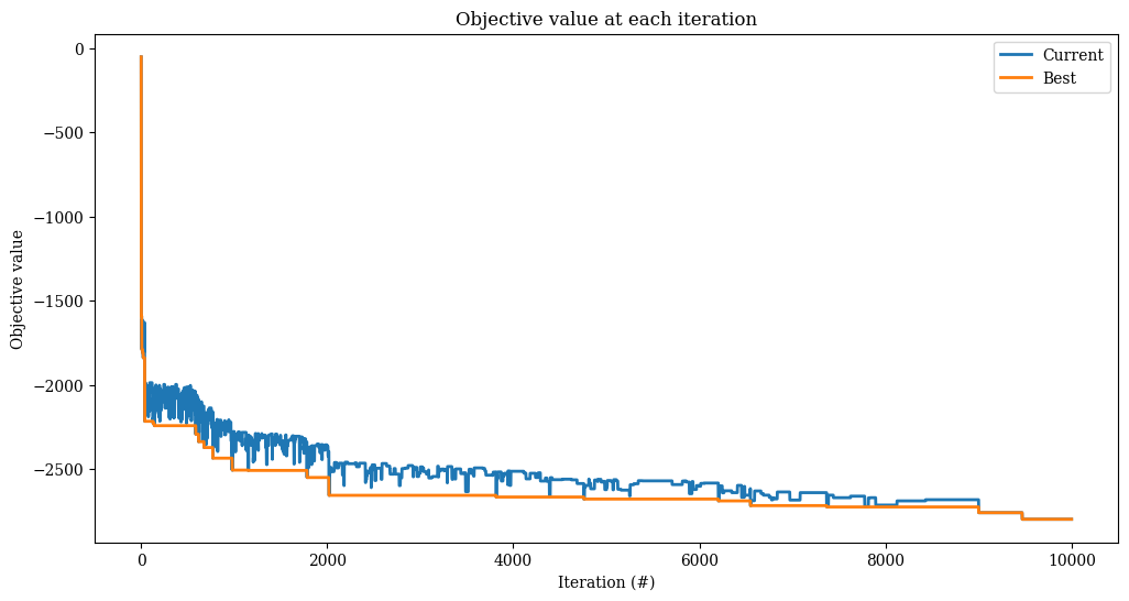
[16]:
select = SegmentedRouletteWheel(
    scores=[5, 2, 1, 0.5],
    decay=0.8,
    seg_length=500,
    num_destroy=2,
    num_repair=1,
)

alns = make_alns()
res = alns.iterate(init_sol, select, accept, MaxIterations(10_000))

print(f"Found solution with objective {-res.best_state.objective()}.")
Found solution with objective 2850.0.
[17]:
_, ax = plt.subplots(figsize=(12, 6))
res.plot_objectives(ax=ax, lw=2)
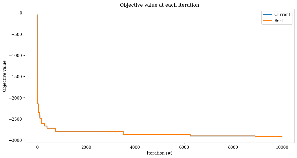
\(\alpha\)-UCB
The \(\alpha\)-UCB scheme is an upper confidence bound bandit algorithm that learns good (destroy, repair) operator pairs, and plays those more often during the search. The \(\alpha\) parameter controls the exploration performed by the learning algorithm: values of \(\alpha\) near one result in much exploration, whereas values of \(\alpha\) nearer to zero result in more exploitation of good operator pairs. Typically, \(\alpha \le 0.1\) is a good choice.
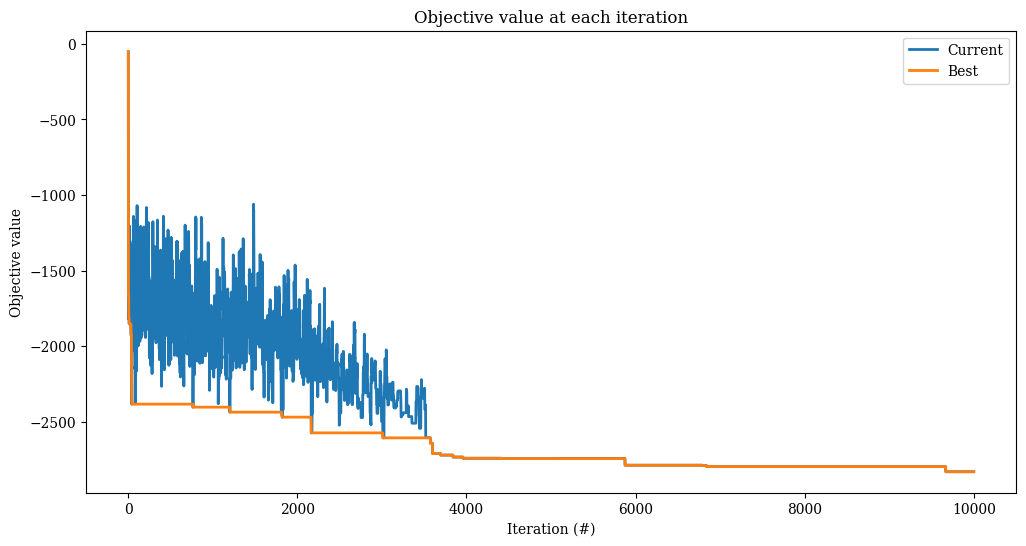
[18]:
select = AlphaUCB(
    scores=[5, 2, 1, 0.5], alpha=0.05, num_destroy=2, num_repair=1
)

alns = make_alns()
res = alns.iterate(init_sol, select, accept, MaxIterations(10_000))

print(f"Found solution with objective {-res.best_state.objective()}.")
Found solution with objective 2849.0.
[19]:
_, ax = plt.subplots(figsize=(12, 6))
res.plot_objectives(ax=ax, lw=2)
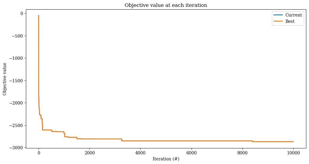
More advanced bandit algorithms
Operator selection can be seen as a multi-armed-bandit problem. Each operator pair is a bandit arm, and the reward for each arm corresponds to the evaluation outcome depending on the score array. Accordingly, any multi-armed bandit algorithm can be used as an operator selection scheme. ALNS integrates with MABWiser to provide access to more bandit algorithms. You may install MABWiser as an extra dependency using pip install alns[mabwiser].
Here, we use a simple epsilon-greedy algorithm from MABWiser. The algorithm picks a random operator pair with probability \(\epsilon=0.15\) and otherwise chooses the operator pair with the largest mean so far.
[20]:
select = MABSelector(
    scores=[5, 2, 1, 0.5],
    num_destroy=2,
    num_repair=1,
    learning_policy=LearningPolicy.EpsilonGreedy(epsilon=0.15),
)

alns = make_alns()
res = alns.iterate(init_sol, select, accept, MaxIterations(10_000))

print(f"Found solution with objective {-res.best_state.objective()}.")
Found solution with objective 2893.0.
[21]:
_, ax = plt.subplots(figsize=(12, 6))
res.plot_objectives(ax=ax, lw=2)
Contextual bandit algorithms
Some MABWiser bandit algorithms require a context vector when making an operator selection choice. To utilize these algorithms, your State class must additionally conform to the ContextualState protocol found in ALNS.State. In practice, this simply means adding an additional method that takes no arguments and returns context data about your state. Here we monkey-patch our existing KnapsackState to conform to the ContextualState protocol.
[22]:
def get_knapsack_context(self: KnapsackState):
    num_items = np.count_nonzero(self.x)
    avg_weight = self.weight() / num_items
    return np.array([self.weight(), num_items, avg_weight])


KnapsackState.get_context = get_knapsack_context
We can now use a contextual bandit algorithm such as LinGreedy. See the MABWiser documentation for more details on how this and other contextual bandit algorithms work.
[23]:
select = MABSelector(
    scores=[5, 2, 1, 0.5],
    num_destroy=2,
    num_repair=1,
    learning_policy=LearningPolicy.LinGreedy(epsilon=0.15),
)

alns = make_alns()
res = alns.iterate(init_sol, select, accept, MaxIterations(10_000))

print(f"Found solution with objective {-res.best_state.objective()}.")
Found solution with objective 2893.0.
[24]:
_, ax = plt.subplots(figsize=(12, 6))
res.plot_objectives(ax=ax, lw=2)
Acceptance criteria
We have just looked at the different weight schemes, using a fixed acceptance criterion. Now we flip this around: we fix an operator selection scheme, and look at several acceptance criteria the alns package offers. Note that this list is not exhaustive: for a look at all available acceptance criteria, head over to alns.accept.
[25]:
select = SegmentedRouletteWheel(
    scores=[5, 2, 1, 0.5],
    decay=0.8,
    seg_length=500,
    num_destroy=2,
    num_repair=1,
)
Hill climbing
This acceptance criterion only accepts better solutions. It was used in the examples explaining the operator selection schemes, so we will not repeat it here. You might also be interested in the other example notebooks for the cutting stock and travelling salesman problems, which also rely on this acceptance criterion.
Record-to-record travel
This criterion accepts solutions when the improvement meets some updating threshold.
In particular, consider the current best solution \(s^*\) with objective \(f(s^*)\). A new candidate solution \(s^c\) is accepted if the improvement \(f(s^c) - f(s^*)\) is smaller than some updating threshold \(t\). This threshold is initialised at some starting value, and then updated using a step value \(u\). There are two ways in which this update can take place:
linear: the threshold is updated linearly, as \(t = t - u\).
exponential: the threshold is updated exponentially, as \(t = t \times u\).
Finally, the threshold \(t\) cannot become smaller than a minimum value, the end threshold.
[26]:
accept = RecordToRecordTravel(
    start_threshold=255, end_threshold=5, step=250 / 10_000, method="linear"
)

alns = make_alns()
res = alns.iterate(init_sol, select, accept, MaxIterations(10_000))

print(f"Found solution with objective {-res.best_state.objective()}.")
Found solution with objective 2890.0.
[27]:
_, ax = plt.subplots(figsize=(12, 6))
res.plot_objectives(ax=ax, lw=2)
Simulated annealing
This criterion accepts solutions when the scaled probability is bigger than some random number, using an updating temperature that drives the probability down. It is very similar to the RecordToRecordTravel criterion, but uses a different acceptance scheme.
In particular, a temperature is used, rather than a threshold, and the candidate \(s^c\) is compared against the current solution \(s\), rather than the current best solution \(s^*\). The acceptance probability is calculated as
where \(t\) is the current temperature.
[28]:
accept = SimulatedAnnealing(
    start_temperature=1_000,
    end_temperature=1,
    step=1 - 1e-3,
    method="exponential",
)

alns = make_alns()
res = alns.iterate(init_sol, select, accept, MaxIterations(10_000))

print(f"Found solution with objective {-res.best_state.objective()}.")
Found solution with objective 2858.0.
[29]:
_, ax = plt.subplots(figsize=(12, 6))
res.plot_objectives(ax=ax, lw=2)
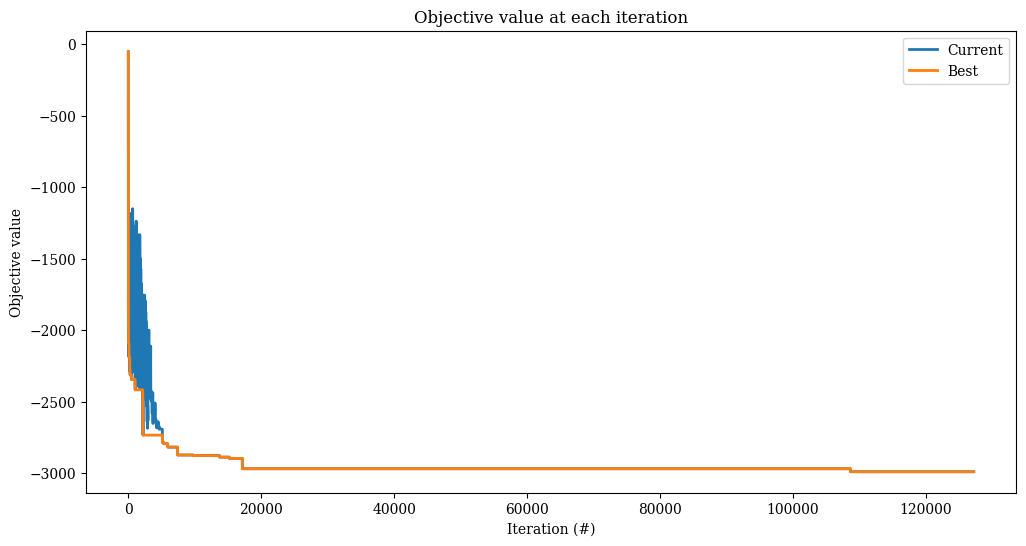
Rather than a fixed number of iterations, we can also fix the runtime, and allow as many iterations as fit in that timeframe.
[30]:
accept = SimulatedAnnealing(
    start_temperature=1_000,
    end_temperature=1,
    step=1 - 1e-3,
    method="exponential",
)

alns = make_alns()
res = alns.iterate(init_sol, select, accept, MaxRuntime(60))  # one minute

print(f"Found solution with objective {-res.best_state.objective()}.")
Found solution with objective 2978.0.
[31]:
_, ax = plt.subplots(figsize=(12, 6))
res.plot_objectives(ax=ax, lw=2)
Other stopping criteria are available in alns.stop.
Conclusions
This notebook has shown the various operator selection schemes, acceptance and stopping criteria that can be used with the alns package. The alns package is designed to be flexible, and it is easy to add new schemes and criteria yourself, by subclassing alns.select.OperatorSelectionScheme, alns.accept.AcceptanceCriterion, or alns.stop.StoppingCriterion.